Tutorial#
This tutorial introduces users to crowsetta.
Finding out what annotation formats are built in to crowsetta#
The first thing we need to do to work with any Python library is import it.
import crowsetta
Now we can use the crowsetta.formats.as_list() function to find out what formats are
built in to Crowsetta.
crowsetta.formats.as_list()
['aud-bbox',
 'aud-seq',
 'birdsong-recognition-dataset',
 'generic-seq',
 'notmat',
 'raven',
 'simple-seq',
 'textgrid',
 'timit',
 'yarden']
Getting some example data to work with#
Since crowsetta is a tool to working with annotations of vocalizations, we need some audio files containing vocalizations that are annotated.
We download some examples of annotation files in the Audacity LabelTrack format, from the dataset “Labeled songs of domestic canary M1-2016-spring (Serinus canaria)” by Giraudon et al., 2021.
!curl --no-progress-meter -L 'https://zenodo.org/record/6521932/files/M1-2016-spring_audacity_annotations.zip?download=1' -o './data/M1-2016-spring_audacity_annotations.zip'
import shutil
shutil.unpack_archive('./data/M1-2016-spring_audacity_annotations.zip', './data/giraudon-et-al-2021')
We use pathlib from the Python standard library to
get a list of those files.
import pathlib
audseq_paths = sorted(pathlib.Path('./data/giraudon-et-al-2021/audacity-annotations').glob('*.txt'))

print(f'There are {len(audseq_paths)} Audacity LabelTrack .txt files')
first_five = "\n".join([str(path) for path in audseq_paths[:5]])
print(f'The first five are:\n{first_five}')
There are 459 Audacity LabelTrack .txt files
The first five are:
data/giraudon-et-al-2021/audacity-annotations/100_marron1_May_24_2016_62101389.audacity.txt
data/giraudon-et-al-2021/audacity-annotations/101_marron1_May_24_2016_64441045.audacity.txt
data/giraudon-et-al-2021/audacity-annotations/102_marron1_May_24_2016_69341205.audacity.txt
data/giraudon-et-al-2021/audacity-annotations/103_marron1_May_24_2016_73006746.audacity.txt
data/giraudon-et-al-2021/audacity-annotations/104_marron1_May_24_2016_73006746.audacity.txt
Using the Transcriber to load annotation files#
Now we want to use crowsetta to load the annotations from files.
First we get all the annotation files in some variable.
(We have already done this using pathlib.Path.glob above.)
Now we use crowsetta.Transcriber to load them.
The Transcriber is a Python class, and we want to create a new
instance of that class. You don’t have to understand what that
means, but you do have to know that before you can do anything with a
Transcriber, you have to call the class, as if it were a function,
and assign it to some variable, like this:
scribe = crowsetta.Transcriber(format='aud-seq')
print("scribe is an instance of a", type(scribe))
scribe is an instance of a <class 'crowsetta.transcriber.Transcriber'>
Now we have a scribe with methods that we can use on our
annotation files (methods are functions that “belong” to a class).
We use the from_file method of the Transcriber to load the annotations.
audseqs = []

for audseq_path in audseq_paths:
    audseqs.append(scribe.from_file(audseq_path))


print(f'There are {len(audseqs)} Audacity LabelTrack annotations')
print(f'The first one looks like:\n{audseqs[0]}')
There are 459 Audacity LabelTrack annotations
The first one looks like:
AudSeq(start_times=array([ 0.        ,  0.35      ,  0.664     ,  1.359     ,  2.412     ,
        2.488     ,  2.773     ,  2.83498145,  2.969     ,  4.398     ,
        4.695     ,  4.835     ,  5.69797655,  6.768     ,  6.925     ,
        7.059     ,  7.104     ,  8.009     ,  8.432     ,  8.617     ,
        9.463     , 10.24179069, 10.77685142, 11.469     , 11.53      ,
       12.281     , 13.603     , 13.645     , 15.36268604, 15.5305959 ,
       15.562     , 17.088     , 18.52      , 18.581     , 18.75233777,
       18.831     , 19.66      , 19.73      , 19.744     , 19.907     ,
       19.974     , 20.304     , 20.408     , 20.688     , 21.007     ,
       21.049     , 22.643     , 22.663     , 24.879     , 25.039     ,
       25.064     , 26.145     , 27.591     , 27.652     , 27.834     ,
       27.958     , 28.947     , 29.        , 29.199     , 29.257     ,
       29.591     , 29.703     , 29.92698303, 31.52095975, 31.535     ,
       31.697     , 31.838     , 32.46501978, 32.468     , 32.538     ,
       32.636     , 33.546     , 34.521     , 34.566     , 36.7623138 ,
       36.802     , 37.712     ]), end_times=array([ 0.35      ,  0.664     ,  1.359     ,  2.412     ,  2.488     ,
        2.773     ,  2.83498145,  2.969     ,  4.398     ,  4.695     ,
        4.835     ,  5.69797655,  6.77089937,  6.925     ,  7.059     ,
        7.104     ,  8.009     ,  8.432     ,  8.617     ,  9.463     ,
       10.24179069, 10.78245415, 11.469     , 11.53      , 12.281     ,
       13.603     , 13.645     , 15.382     , 15.5305959 , 15.562     ,
       17.088     , 18.52      , 18.581     , 18.75233777, 18.831     ,
       19.66      , 19.73      , 19.744     , 19.907     , 19.974     ,
       20.304     , 20.408     , 20.688     , 21.007     , 21.049     ,
       22.643     , 22.663     , 24.879     , 25.039     , 25.064     ,
       26.145     , 27.591     , 27.652     , 27.834     , 27.958     ,
       28.947     , 29.        , 29.199     , 29.257     , 29.591     ,
       29.703     , 29.927     , 31.52095975, 31.535     , 31.697     ,
       31.838     , 32.46501978, 32.468     , 32.538     , 32.636     ,
       33.546     , 34.521     , 34.566     , 36.7623138 , 36.802     ,
       37.712     , 37.779     ]), labels=<StringArray>
[ 'SIL', 'call',  'SIL',    'Z',  'SIL',    'T',  'SIL',  'SIL',    'U',
   'J2',  'SIL',   'B1',   'B2',    'R',  'SIL',   'J1',   'J1',   'J2',
  'SIL',   'B1',   'B2',    'Q',    'O',  'SIL',   'J1',    'L',  'SIL',
    'N',    'S',  'SIL',    'M',    'D',  'SIL',    'I',  'SIL',    'A',
    'A',  'SIL',    'O',  'SIL',    'P',  'SIL',    'K',   'K2',  'SIL',
    'L',  'SIL',    'N',    'S',  'SIL',    'M',    'D',  'SIL',    'I',
  'SIL',    'A',  'SIL',    'O',  'SIL',    'P',  'SIL',    'K',    'V',
  'SIL',    'O',  'SIL',   'J1',  'SIL',   'J2',  'SIL',   'B1',   'B2',
  'SIL',    'N',  'SIL',    'A',    'A']
Length: 77, dtype: string, annot_path=PosixPath('data/giraudon-et-al-2021/audacity-annotations/100_marron1_May_24_2016_62101389.audacity.txt'), notated_path=None)
Using the to_annot method to convert annotations into data types we can work with in Python#
Now that we have loaded the annotations, we want to get them into some
data type that makes it easier to get what we want out of the annotated files
(in this case, audio files).
Just like Python has data types like a list or dict that make it
easy to work with data, crowsetta provides data types meant to
work with many different formats.
For any format built into crowsetta, we can convert the annotations
that we load into a generic crowsetta.Annotation (or a list of
Annotations, if a single annotation file contains annotations
for multiple annotated audio files or spectrograms).
annots = []
for audseq in audseqs:
    annots.append(scribe.from_file(audseq_path).to_annot())
print(f'The first Annotation: {annots[0]}')
The first Annotation: Annotation(annot_path=PosixPath('data/giraudon-et-al-2021/audacity-annotations/558_marron1_May_23_2016_67003910.audacity.txt'), notated_path=None, seq=<Sequence with 42 segments>)
Depending on the format type, sequence-like
or bounding box-lie,
the Annotation will either have a seq attribute,
short for “Sequence”, or a bbox attribute,
short for “Bounding box”.
Since 'aud-seq' is a sequence-like format,
the Annotations have a seq attribute:
print(
    f'seq for first Annotation: {annots[0].seq}'
)
seq for first Annotation: <Sequence with 42 segments>
The two types of formats each have their own
corresponding data type, crowsetta.Sequence and crowsetta.BBox
These are the data types that make it easier to work with your annotations.
We work more with Sequences below.
But first we mention a couple other features of Annotations.
When we convert the annotation to a generic crowsetta.Annotation,
we retain the path to the original annotation file,
in the attribute annot_path,
and we optionally have the path to the file that it annotates, notated_path.
print(
    f'annot_path for first Annotation: {annots[0].annot_path}'
)
annot_path for first Annotation: data/giraudon-et-al-2021/audacity-annotations/558_marron1_May_23_2016_67003910.audacity.txt
Notice that we can chain the methods from_file and to_annot
to make loading the annotations and converting them
to generic crowsetta.Annotations into a one-liner:
annots = []
for audseq_path in audseq_paths:
    annots.append(scribe.from_file(audseq_path).to_annot())
We didn’t do this above, just because we wanted to introduce the methods one-by-one.
Working with Sequences#
As we said, what we really want is some data types that make it easier to work with our annotations, and that help us write clean, readable code.
The Audacity .txt format
we are using in this tutorial above is one of what
crowsetta calls a “sequence-like” format,
as stated above.
What this means is that we can convert our
each one of our 'aud-seq' annotations to
a Sequence.
Each Sequence consists of some number of Segments, i.e., a
part of the sequence defined by an onset and offset that has a
label associated with it.
These Sequences and Segments are what specifically helps
us write clean code, as we’ll see below.
(Bounding box-like annotation formats similarly give us generic
crowsetta.BBoxs that we can use to write code.)
Since we have already created the crowsetta.Annotations,
we can make a list of crowsetta.Sequences from them
by just grabbing the Sequence of each Annotation.
seqs = []
for annot in annots:
    seqs.append(annot.seq)
Notice again that we could have done this as a one-liner,
using the to_seq method to load each file into a Sequence.
(but we didn’t, because we wanted to explain the different methods to you):
seqs = []
for audseq_path in audseq_paths:
    seqs.append(scribe.from_file(audseq_path).to_seq())
Each sequence-like format has a to_seq method,
and each bounding box-like format has a to_bbox method.
When you call to_annot, that method actually calls to_seq
or to_bbox when creating the crowsetta.Annotations.
But if you just need those data types, without the metadata
provided by an Annotation,
you can get them directly by calling the method yourselves.
For each annotation file, we should now have a Sequence.
print("Number of annotation files: ", len(audseq_paths))
print("Number of Sequences: ", len(seqs))
if len(audseq_paths) == len(seqs):
    print("The number of annotation files is equal to number of sequences.")
Number of annotation files:  459
Number of Sequences:  459
The number of annotation files is equal to number of sequences.
print("first element of seqs: ", seqs[0])
print("\nFirst two Segments of first Sequence:")
for seg in seqs[0].segments[0:2]: print(seg)
first element of seqs:  <Sequence with 77 segments>

First two Segments of first Sequence:
Segment(label='SIL', onset_s=np.float64(0.0), offset_s=np.float64(0.35), onset_sample=None, offset_sample=None)
Segment(label='call', onset_s=np.float64(0.35), offset_s=np.float64(0.664), onset_sample=None, offset_sample=None)
Using crowsetta data types to write clean code#
Now that we have a list of Sequences, we can iterate
(loop) through it to get at our data in a clean, Pythonic way.
Let’s say we’re interested in the number of occurrences of each class in our dataset, in this case, different phrases of the canary’s song as well as some other sounds, like calls. We also want to inspect the distribution of durations of each of these classes.
To achieve this, we will create a pandas.Dataframe
and then plot distributions of the data in that Dataframe with seaborn.
We loop over all the Sequences, and then in an inner
loop, we’ll iterate through all the Segments in each
Sequence, grabbing the label property from the Segment
so we know what class it is,
and computing the duration by subtracting
the onset time from the offset time.
import pandas as pd

records = []

for sequence in seqs:
    for segment in sequence.segments:
        records.append(
            {
                'label': segment.label,
                'duration': segment.offset_s - segment.onset_s
            }
        )

df = pd.DataFrame.from_records(records)
from IPython.display import display
display(df.head(10))
| label | duration | |
|---|---|---|
| 0 | SIL | 0.350 |
| 1 | call | 0.314 |
| 2 | SIL | 0.695 |
| 3 | Z | 1.053 |
| 4 | SIL | 0.076 |
| 5 | T | 0.285 |
| 6 | SIL | 0.062 |
| 7 | SIL | 0.134 |
| 8 | U | 1.429 |
| 9 | J2 | 0.297 |
(There are more concise ways to do that, but doing it the way we did let
us clearly see iterating through the Segments and
Sequences.)
import matplotlib.pyplot as plt
import seaborn as sns
sns.set_context("paper")
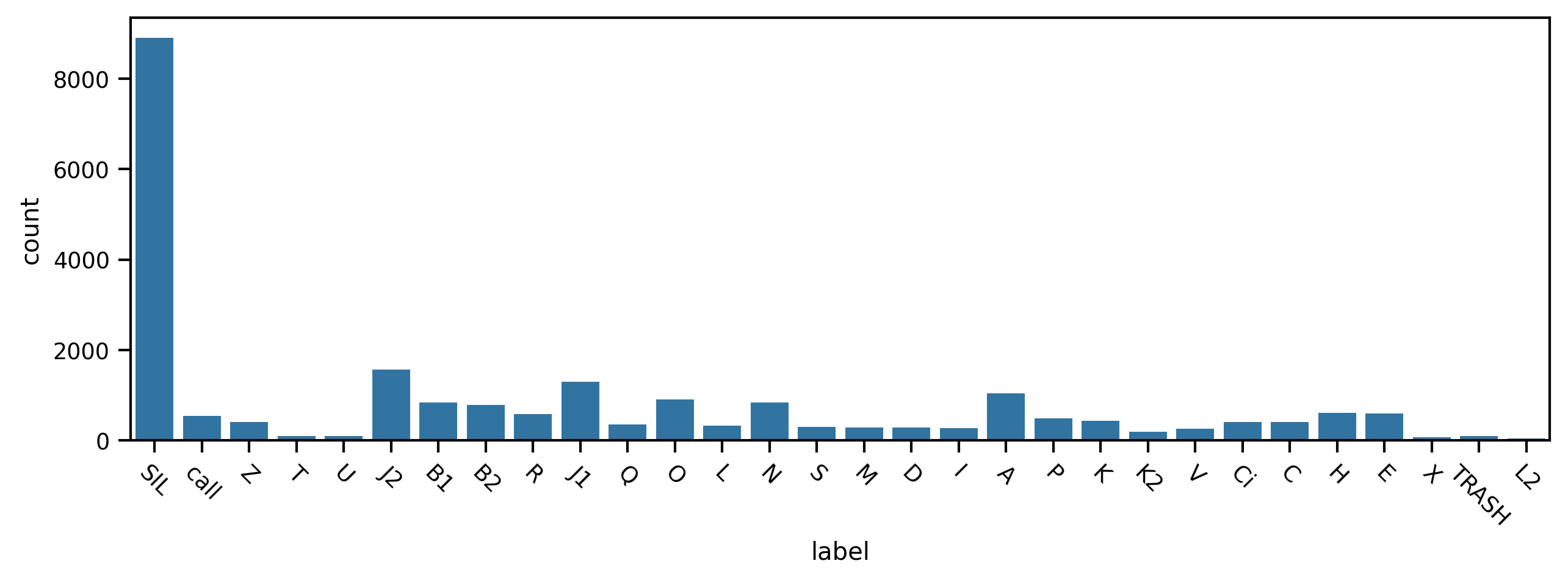
First we plot the counts for each phrase type. We notice there are many more silent periods (“SIL”) and observe some smaller differences between the phrases themselves.
fig, ax = plt.subplots(figsize=(10,3), dpi=300)
sns.countplot(data=df, x='label', ax=ax)
ax.set_xticklabels(ax.get_xticklabels(),rotation = -45);
/tmp/ipykernel_1031/3763166274.py:3: UserWarning: set_ticklabels() should only be used with a fixed number of ticks, i.e. after set_ticks() or using a FixedLocator.
  ax.set_xticklabels(ax.get_xticklabels(),rotation = -45);
Now let’s find the three most frequently-occurring phrases and examine the distributions of their durations. We ignore the silent periods.
df = df[df['label'] != 'SIL']  # remove silent periods
counts = df['label'].value_counts()  # get the counts of the labels
most_frequent = counts[:3].index.values.tolist()  # find the top 3 most frequent
df = df[df['label'].isin(most_frequent)]  # keep those top 3 most frequent in the original DataFrame
sns.set(font_scale=2)
sns.displot(data=df, x='duration', col='label', hue='label', col_wrap=3)
<seaborn.axisgrid.FacetGrid at 0x75c70bdf1160>
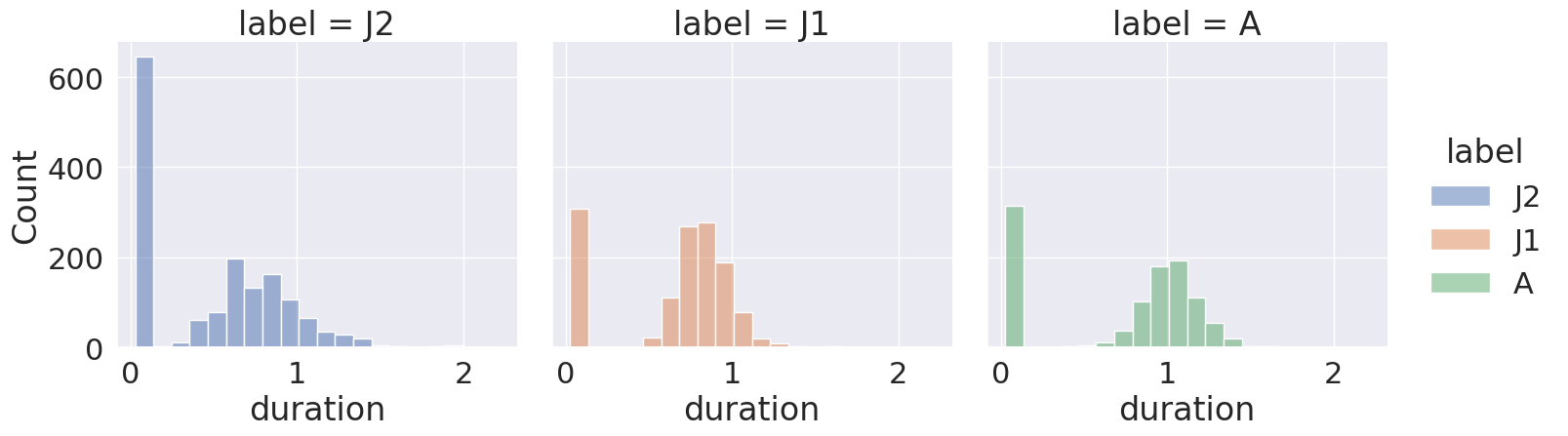
We can see that each phrase has a roughly similar distribution of durations. We also notice that for each phrase type there’s one bin containing many very short durations, that we may want to inspect more closely in our data, to better understand how they arise. (This is one example of why it’s always a good idea to visualize the descriptive statistics of any dataset you work with.)
Okay, now you’ve seen the basics of working with crowsetta. Get out there and analyze some vocalizations!