Munging annotations from Praat TextGrid files with crowsetta to fit a first-order Markov model of birdsong syntax

A common need when working with annotations for animal vocalizations is to transform them to perform a certain analysis. This is a sort of data munging. In this vignette, we provide a simple example of munging annotations to build a model of birdsong syntax.

We will work with a dataset of Bengalese finch song annotated in a format used by “evsonganaly”, a MATLAB GUI for annotating song. We want to build a matrix of the transition probabilities between syllables in the song, that is, a first-order Markov model.

Download this page as a Jupyter notebook!

To work with this tutorial interactively, we suggest downloading this notebook! Click on the download icon in the upper right to download a Markdown file (with ‘.md’ extension) that you can run as a Jupyter notebook after installing Jupyter lab and jupytext.

Workflow

Here’s the steps we’ll follow:

0. Write code for analysis

1. Load .not.mat files saved by evsonganaly with crowsetta, and convert to crowsetta Annotations with Sequences

2. Munge data

3. Compute transition matrices

For this vignette, we use annotations from the Bengalese finch song repository, by Nicholson, Queen, Sober 2017 [1], adapted under CC BY 4.0 License.

0. Write code for analysis

Before we can analyze our data, we need to know what analysis we’re doing. It can save you a lot of time to write a rough draft of this analysis code first, and test it with some toy data that you generate.

We also do this first to help understand what format we’re going to need to get our data into below.

Our goal here is to fit a first-order Markov model of the transition probabilities in the song of Bengalese finches. This model has been used in several previous studies[2][3], although it was later shown[4] that such a model does not completely describe the statistics of the song. In spite of that, a first-order Markov model is very convenient to fit, and can give us a useful first-order approximation (literally!) of singing behavior.

To build such a model for Bengalese finch song, we consider the song syllables to be states. We construct a transition matrix \(P\) where the rows are the state we’re transitioning from, the columns are the state we’re transitioning to, and thus the value in each cell \(p_{i, j}\) is the probability of transitioning from state \(i\) to state \(j\). We construct this matrix given a set of sequences \(X\), where each sequence \(x_t\) is a chain of states from a set \(S\), which in our case will be the set of syllable labels. To construct the matrix, we count the number of occurrences of each of the possible pairwise transitions from one state to another. Then, to compute the probabilities, we divide the counts for each pair by the total number of transitions. To replicate the approach used in [3], we will add start and end states to our transition matrix, that correspond to the start and end of each song bout, instead of computing a separate vector of initial state probabilities \(P_{init}\).

We will write a “pipeline” to compute this, which has basically two steps.

1. Using annotations loaded into crowsetta, get the unique set of states, and the counts of every occurrence of transitioning from one state to another.

2. Use the states and counts to compute the probabilities for the first-order Markov model

We write functions for step 1 and 2 below.
The functions are written in such a way that, after cleaning and transforming our loaded annotations, we pass them into the second function, and it will call the first one for us when it computes the transition matrix.

Note

This code is adapted from yardencsGitHub/tweetynet under BSD license.

As used for the paper Cohen, Y., Nicholson, D., Sanchioni, A., Mallaber, E., Skidanova, V., & Gardner, T. (2022). Automated annotation of birdsong with a neural network that segments spectrograms. eLife. https://doi.org/10.7554/eLife.63853

"""functions for analyzing sequences of Bengalese finch syllable labels"""
from __future__ import annotations
from collections import Counter, namedtuple

import crowsetta
import numpy as np


def states_and_counts_from_labels(labels: list[np.ndarray],
                                  start_state:str = '@', 
                                  end_state:str = '!') -> set:
    """Get ``states`` and ``counts``
    from a list of numpy arrays of string characters, 
    to build a transition matrix
    showing the probability of going from
    one state to another.

    Parameters
    ----------
    labels : list
        Of numpy.ndarray of string labels, 
        taken from the ``Sequence.label`` 
        attributes of ``crowsetta.Annotation`` instances.
        Will be used to count transitions
        from one label to another
        in the sequences of syllables.
    start_state : str
        Single character used to indicate the 
        start of a bout of song. Default is '@'.
    end_state : str
        Single character used to indicate the 
        end of a bout of song. Default is '!'.

    Returns
    -------
    states : set
        of characters, set of
        unique labels
        that occur in the list of
        ``Annotation``s.
    counts : collections.Counter
        where keys are transitions
        of the form "from label,
        to label", e.g. "ab",
        and values are number of
        occurrences of that transition.

    Notes
    -----
    Note that characters for start and end states 
    are appended to the beginning and end of 
    each string in ``labels`` to build the 
    transition matrix as in Jin Kozhevnikov 2011.
    """
    # make sequences with start and end states
    seqs = []
    for seq_labels in labels:
        seq_labels = np.concatenate((np.array([start_state]), seq_labels, np.array([end_state])))
        seqs.append(seq_labels)

    # set of (unique) states
    states = sorted(
        set([state
             for seq in seqs
             for state in seq
             ])
    )

    counts = Counter()
    for seq in seqs:
        transitions = zip(seq[:-1], seq[1:])
        for transition in transitions:
            counts[transition] += 1

    return states, counts


def row_norm(mat: np.ndarray) -> np.ndarray:
    """Normalize matrix rows, so they sum to one"""
    return mat / mat.sum(axis=1)[:, np.newaxis]


TransitionMatrix = namedtuple('TransitionMatrix',
                              field_names=('counts',
                                           'matrix',
                                           'states'))


def transmat_from_labels(labels: list[np.ndarray],
                         thresh: float | None = None,
                         start_state:str = '@', 
                         end_state:str = '!') -> TransitionMatrix:
    """From list of labels from ``crowsetta.Annotation``s,
    returns ``TransitionMatrix`` tuple with fields
    'counts', 'matrix', and 'states'

    Parameters
    ----------
    labels : list
        Of numpy.ndarray of string labels, 
        taken from the ``Sequence.label`` 
        attributes of ``crowsetta.Annotation`` instances.
        Will be used to count transitions
        from one label to another
        in the sequences of syllables.
    thresh : float
        threshold used to smooth probabilities.
        If not None, any probabilities less
        than threshold are set to 0.0 and then
        the transition matrix is again row
        normalized
    start_state : str
        Single character used to indicate the 
        start of a bout of song. Default is '@'.
    end_state : str
        Single character used to indicate the 
        end of a bout of song. Default is '!'.

    Returns
    -------
    trans_mat : TransitionMatrix
        A NamedTuple with fields 'counts', 'matrix', and 'states'.

    Notes
    -----
    Note that characters for start and end states 
    are appended to the beginning and end of 
    each string in ``labels`` to build the 
    transition matrix as in Jin Kozhevnikov 2011.
    
    The returned matrix will have (:math:`s - 1` rows 
    and :math:`s` columns, where :math`s` is the 
    number of states, (i.e., ``len(trans_mat.states)``).
    This is because there is no probability 
    of transitioning from the end state to any other.
    """
    states, counts = states_and_counts_from_labels(labels, start_state=start_state, end_state=end_state)

    counts_arr = np.array(
        [[counts[i, j] for j in states] for i in states], dtype=float
    )

    # remove row for end state since probability of 
    # transitioning *from* that state to any other is zero.
    # we use a mask to keep only rows we want
    end_state_ind = states.index(end_state)
    rows = np.ones(counts_arr.shape[0], dtype=bool)
    rows[end_state_ind] = False
    counts_arr = counts_arr[rows]

    trans_mat = row_norm(counts_arr)
    if thresh is not None:
        trans_mat[trans_mat < thresh] = 0.0
        trans_mat = row_norm(trans_mat)

    return TransitionMatrix(counts=counts, matrix=trans_mat, states=states)

1. Load data with crowsetta

We change directories so we can access the ./data directory we have set up for our project, following good practices.

cd ..

/home/docs/checkouts/readthedocs.org/user_builds/crowsetta/checkouts/latest/doc

/home/docs/checkouts/readthedocs.org/user_builds/crowsetta/envs/latest/lib/python3.10/site-packages/IPython/core/magics/osm.py:417: UserWarning: using dhist requires you to install the `pickleshare` library.
  self.shell.db['dhist'] = compress_dhist(dhist)[-100:]

Our TextGrid files are in a sub-directory, ./data/r6pqa (the unique ID associated with the OSF project for the dataset).

We get a list of the TextGrid files from that subdirectory using pathlib.

To download these files and work with them locally, click the following links: b06_concat_dtw.TextGrid
b11_concat_dtw.TextGrid b35_concat_dtw.TextGrid

import pathlib

downloaded_dir = pathlib.Path('./data/r6paq/')

We make sure that our paths are sorted just in case it matters for our analysis.

textgrid_paths = sorted(downloaded_dir.glob('*.TextGrid'))

We inspect the first four paths just to check that we got what we expect.

textgrid_paths

[PosixPath('data/r6paq/b06_concat_dtw.TextGrid'),
 PosixPath('data/r6paq/b11_concat_dtw.TextGrid'),
 PosixPath('data/r6paq/b35_concat_dtw.TextGrid')]

Looks like it.

Each of the files corresponds to all the song from one individual bird. E.g., the file b06_concat_dtw.TextGrid contains annotations from the bird with ID “b06” and the file b011_concat_dtw.TextGrid contains annotations from the bird with ID “b11”.

We will need to do some book-keeping as we transform our data so we that we’re able to fit a model for each bird. Mainly this will involve using Python dictionaries where the bird’s ID is the key, and pandas DataFrames where we have the ID in a column.

But first let’s load all those annotations with crowsetta to get a sense of them.

import crowsetta

scribe = crowsetta.Transcriber(format='textgrid')

Notice below the argument keep_empty=True. The parameter keep_empty defaults to False, but we actually want to keep the unlabeled intervals between syllables, because they will help us divide the song up into bouts, as we will see below.

These are large files (that concatenate annotations across a day of song for each bird) so they take a while to load.

textgrids = {}

for textgrid_path in textgrid_paths:
    bird_id = textgrid_path.name.split('_')[0]  # bird ID will be first element from list after split
    annot = scribe.from_file(textgrid_path, keep_empty=True)
    textgrids[bird_id] = annot

2. Munge data

Now we want to munge the data into the format we want to carry out our analysis.

Looking at descriptive statistics

A good first thing to do with any new dataset is plot some descriptive statistics to get an overview of the data before we do anything with it. As an example of this, let’s look at the counts of the different classes of labels.

First we convert the TextGrid annotations to crowsetta.Annotations to make them easier to work with.
Here we use a dictionary comprehension to transform our textgrids dictionary to a dictionary of crowsetta.Annotations.

annots = {bird_id: textgrid.to_annot() 
          for bird_id, textgrid in textgrids.items()}

Now we count the distribution of labels. We loop over the dictionary values since for now we don’t care as much about the labels on a bird-by-bird basis (you’ll see why after we inspect them).

from collections import Counter

counts = Counter(
    [lbl for annot in annots.values() for lbl in annot.seq.labels]
)

print(counts)

Counter({'': 53428, 'x': 20970, 'd': 4924, 'e': 4520, 'b': 3992, 'c': 3896, 'a': 3807, 'f': 2878, 'g': 2147, 'h': 1524, 'l': 1209, 'j': 1203, 'k': 1200, 'i': 1158})

We can see that we have many segments in our sequences that have the label 'x'. These are squawky “intro” notes that are sometimes ommitted from models of song syntax.

In fact this is the most frequent label! (The collection.Counter prints its key-value pairs in descending order of value by default.)

We will remove the squawky “intro” notes for this analysis (this is sometimes called “cleaning” data, although maybe you shouldn’t make your data feel like it’s dirty).

Dividing the annotations into song bouts

We want to add states to our model for the beginning and ending of each song bout. To do that with the data we’re using here, we need to find the bouts within the annotations somehow, since each annotation file contains entire days of song.

One way to do this is to set a threshold on the duration of silent intervals, e.g. greater than 500 seconds, and use that threshold to break up annotations into bouts.

Before we do that, let’s eyeball the distribution of the silent intervals with empty string labels, to see what kind of threshold might make sense.

We start by converting the annotations to a pandas.DataFrame so we can easily munge and tidy the data. This is one advantage of moving from the Praat TextGrid format to the 'generic-seq' format built into crowsetta.

One approach would be to put all the annotations in a single DataFrame, adding a column named 'bird ID' that we’d use to split the DataFrame back up below (a sort of “long form” DataFrame). But we’ll stick with a dictionary to hopefully make the loops a bit easier to follow without inspecting the contents of DataFrames. Our new dictionary dfs will map each bird ID to a pandas.DataFrame made from its annotations.

dfs = {
    bird_id: crowsetta.formats.seq.GenericSeq(annots=annot).to_df()
    for bird_id, annot in annots.items()
}

for bird_id, df in dfs.items():
    df['duration'] = df['offset_s'] - df['onset_s']

import matplotlib.pyplot as plt

fig, ax_arr = plt.subplots(2, 2, figsize=(10,8), dpi=150)
ax_arr = ax_arr.ravel()

for ax_ind, (bird_id, df) in enumerate(dfs.items()):
    ax = ax_arr[ax_ind]

    if ax_ind < 2:
        bins = 100  # so we don't end up with one giant bin with most values in it
    else:
        bins = None  # default is fine
    
    df[df.label == ''].hist(column='duration', bins=bins, ax=ax)
    ax.set_title(bird_id)
    ax.set_xlabel('duration')

    ax.set_xlim([0, 2])
    rects = ax.patches
    for rect in rects[3:18:2]:
        height = rect.get_height()
        ax.text(rect.get_x() + rect.get_width() / 2, height+0.01, f'{int(height)}',
                ha='center', va='bottom', rotation=-45)

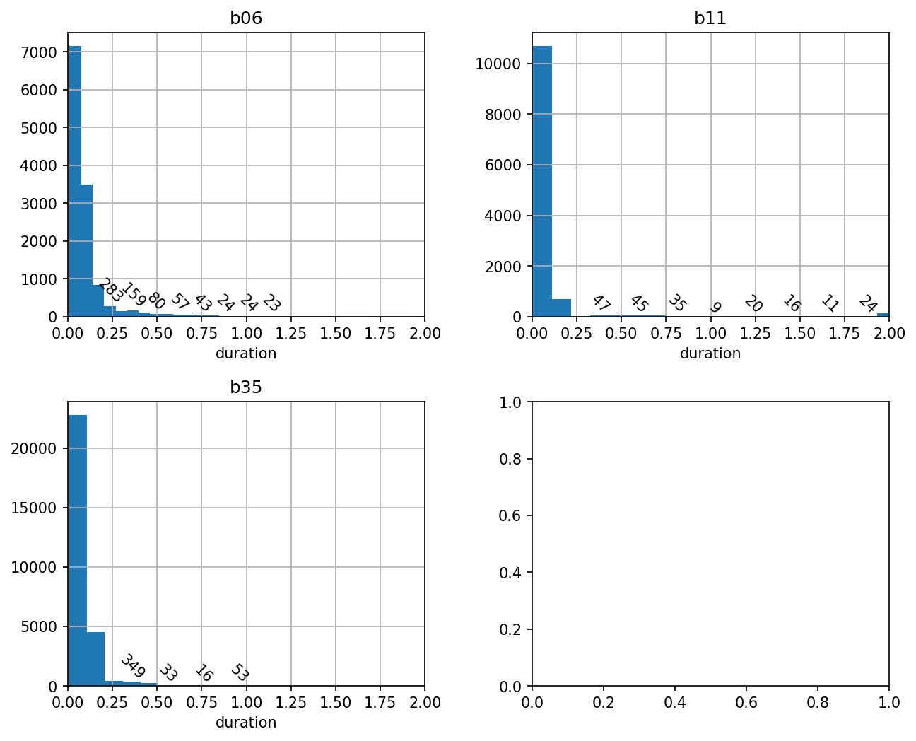
We can see that far and away the most frequent silent intervals are very brief, consistent with what is known about Bengalese finch song, where the silent gaps between syllables are 50-100 ms.

We can also see there’s a long tail of durations that are greater than 500 milliseconds.
To keep this vignette as simple as possible, let’s arbitrarily choose that threshold as “good enough”, and then use it to split our annotations into bouts.

At the same time that we do this, we’ll remove all the other silent labels, which was our goal in the first place.

We continue to work with the pandas.DataFrame for convenience.

First we make a Boolean column that is True where our conditions hold of a segment with a silent label that has a duration greater than our threshold.

THRESHOLD = 0.5

for bird_id, df in dfs.items():
    df['between_bouts'] = (df.duration > THRESHOLD) & (df.label == '')

Now we can find all the places that are True using numpy.nonzero, and then use those indices to split our pandas.DataFrame up into a list of smaller pandas.DataFrame, our bouts. To do the splitting, we use the numpy.array_split function, that can interface with pandas.DataFrames.

import numpy as np

bouts = {}
for bird_id, df in dfs.items():
    inds = np.nonzero(df['between_bouts'].values)[0].tolist()
    bouts_bird = np.array_split(df, inds)
    bouts[bird_id] = bouts_bird

/home/docs/checkouts/readthedocs.org/user_builds/crowsetta/envs/latest/lib/python3.10/site-packages/numpy/core/fromnumeric.py:59: FutureWarning: 'DataFrame.swapaxes' is deprecated and will be removed in a future version. Please use 'DataFrame.transpose' instead.
  return bound(*args, **kwds)

/home/docs/checkouts/readthedocs.org/user_builds/crowsetta/envs/latest/lib/python3.10/site-packages/numpy/core/fromnumeric.py:59: FutureWarning: 'DataFrame.swapaxes' is deprecated and will be removed in a future version. Please use 'DataFrame.transpose' instead.
  return bound(*args, **kwds)
/home/docs/checkouts/readthedocs.org/user_builds/crowsetta/envs/latest/lib/python3.10/site-packages/numpy/core/fromnumeric.py:59: FutureWarning: 'DataFrame.swapaxes' is deprecated and will be removed in a future version. Please use 'DataFrame.transpose' instead.
  return bound(*args, **kwds)

Let’s check bouts for one the birds and see how many that gave us.
We use the set of bouts from the last time through the for loop in the cell above, since it’s still hanging out in memory.

len(bouts_bird)

227

Seems like a reasonable number. What do the bouts look like?
Are they all more or less the same length?

bouts_sorted = sorted(bouts_bird, key=lambda bout: len(bout))
for bout in bouts_sorted[:25]:
    print(len(bout))

2
16
22
24
24
30
30
30
30
34
40
40
40
42
42
48
48
48
52
52
56
56
62
62
64

Hmm, the first few look quite short. Let’s inspect one.

bouts_bird[1]

	label	onset_s	offset_s	notated_path	annot_path	sequence	annotation	duration	between_bouts
260		20.829	21.678	None	data/r6paq/b35_concat_dtw.TextGrid	0	0	0.849	True
261	x	21.678	21.730	None	data/r6paq/b35_concat_dtw.TextGrid	0	0	0.052	False
262		21.730	21.818	None	data/r6paq/b35_concat_dtw.TextGrid	0	0	0.088	False
263	x	21.818	21.904	None	data/r6paq/b35_concat_dtw.TextGrid	0	0	0.086	False
264		21.904	22.002	None	data/r6paq/b35_concat_dtw.TextGrid	0	0	0.098	False
...	...	...	...	...	...	...	...	...	...
537	i	45.523	45.580	None	data/r6paq/b35_concat_dtw.TextGrid	0	0	0.057	False
538		45.580	45.599	None	data/r6paq/b35_concat_dtw.TextGrid	0	0	0.019	False
539	j	45.599	45.670	None	data/r6paq/b35_concat_dtw.TextGrid	0	0	0.071	False
540		45.670	45.707	None	data/r6paq/b35_concat_dtw.TextGrid	0	0	0.037	False
541	k	45.707	45.850	None	data/r6paq/b35_concat_dtw.TextGrid	0	0	0.143	False

282 rows × 9 columns

We can see the one above begins with has many of the silent intervals or the ‘x’ class that we don’t care about. We can filter these intervals out and then inspect our bouts again.

How about a longer DataFrame with more rows in it, though?

bouts_sorted[-1]

	label	onset_s	offset_s	notated_path	annot_path	sequence	annotation	duration	between_bouts
49042		4314.169	4314.670	None	data/r6paq/b35_concat_dtw.TextGrid	0	0	0.501	True
49043	x	4314.670	4314.697	None	data/r6paq/b35_concat_dtw.TextGrid	0	0	0.027	False
49044		4314.697	4314.900	None	data/r6paq/b35_concat_dtw.TextGrid	0	0	0.203	False
49045	x	4314.900	4314.962	None	data/r6paq/b35_concat_dtw.TextGrid	0	0	0.062	False
49046		4314.962	4315.110	None	data/r6paq/b35_concat_dtw.TextGrid	0	0	0.148	False
...	...	...	...	...	...	...	...	...	...
51491	e	4518.538	4518.647	None	data/r6paq/b35_concat_dtw.TextGrid	0	0	0.109	False
51492		4518.647	4518.694	None	data/r6paq/b35_concat_dtw.TextGrid	0	0	0.047	False
51493	f	4518.694	4518.814	None	data/r6paq/b35_concat_dtw.TextGrid	0	0	0.120	False
51494		4518.814	4518.859	None	data/r6paq/b35_concat_dtw.TextGrid	0	0	0.045	False
51495	x	4518.859	4518.933	None	data/r6paq/b35_concat_dtw.TextGrid	0	0	0.074	False

2454 rows × 9 columns

This looks more like a real bout of song, with labels corresponding to the syllables we are interested in. But we still also have silent periods and our ‘x’ segments as well.

Let’s definitely filter all the rows out that are unlabeled, as we set out to do, and the rows where the label is ‘x’ too.

bouts_filtered = {}

for bird_id, bouts_bird in bouts.items():
    bouts_bird = [
        bout[(bout.label != '') & (bout.label != 'x').copy()]
        for bout in bouts_bird
    ]
    bouts_filtered[bird_id] = bouts_bird

After we do that we can inspect our DataFrames again and see if they’re more like sequences of syllables.

for bout in bouts_filtered['b35'][:10]:
    print(len(bout))

83
77
46
109
52
24
30
23
45
20

Not surprisingly they are shorter. There may be some empty “bouts” that we need to discard.
What do the bouts look like after filtering?

bouts_filtered['b35'][3].head()

	label	onset_s	offset_s	notated_path	annot_path	sequence	annotation	duration	between_bouts
737	a	64.726	64.822	None	data/r6paq/b35_concat_dtw.TextGrid	0	0	0.096	False
739	b	64.896	65.019	None	data/r6paq/b35_concat_dtw.TextGrid	0	0	0.123	False
741	c	65.043	65.192	None	data/r6paq/b35_concat_dtw.TextGrid	0	0	0.149	False
743	d	65.220	65.369	None	data/r6paq/b35_concat_dtw.TextGrid	0	0	0.149	False
747	f	65.650	65.762	None	data/r6paq/b35_concat_dtw.TextGrid	0	0	0.112	False

Yes, this actually looks like a sequence of syllables.

Let’s filter out the empty “bouts”.

bouts_filtered = {
    bird_id: [bout for bout in bouts if len(bout) > 0]
    for bird_id, bouts in bouts_filtered.items()
}

Now finally we’ll make new annotated sequences that we can pass to the functions we wrote above.

annots_munged = {}

for bird_id, bouts in bouts_filtered.items():
    annots= []
    for bout in bouts:    
        bout = bout.reset_index()  # so we can get row '0' below
        onsets_s, offsets_s, labels = bout.onset_s.values, bout.offset_s.values, bout.label.values
        seq = crowsetta.Sequence.from_keyword(onsets_s=onsets_s, offsets_s=offsets_s, labels=labels)
        annot_path = bout.loc[0, 'annot_path']  # will be the same for all rows
        annot = crowsetta.Annotation(annot_path=annot_path, seq=seq)
        annots.append(annot)
    annots_munged[bird_id] = annots

So how many bouts did we end up with? We check for one bird.

len(annots_munged['b35'])

223

This is a bit low for four days of song, but good enough number to fit a model for our purposes here.

We inspect the Sequence of the first Annotation just to further confirm that it worked.

annots_munged['b35'][0].seq.segments[:10]

(Segment(label='b', onset_s=1.263, offset_s=1.376, onset_sample=None, offset_sample=None),
 Segment(label='c', onset_s=1.399, offset_s=1.547, onset_sample=None, offset_sample=None),
 Segment(label='d', onset_s=1.572, offset_s=1.716, onset_sample=None, offset_sample=None),
 Segment(label='e', onset_s=1.941, offset_s=2.052, onset_sample=None, offset_sample=None),
 Segment(label='f', onset_s=2.099, offset_s=2.219, onset_sample=None, offset_sample=None),
 Segment(label='g', onset_s=2.249, offset_s=2.351, onset_sample=None, offset_sample=None),
 Segment(label='h', onset_s=2.391, offset_s=2.481, onset_sample=None, offset_sample=None),
 Segment(label='i', onset_s=2.51, offset_s=2.565, onset_sample=None, offset_sample=None),
 Segment(label='j', onset_s=2.582, offset_s=2.655, onset_sample=None, offset_sample=None),
 Segment(label='k', onset_s=2.684, offset_s=2.814, onset_sample=None, offset_sample=None))

Yes, this looks like what we saw in the DataFrame above, converted to annotations.

We have now transformed the annotations into the format we want for our analysis. This is a point in our analysis pipeline where we go from one form of the data for another, so it’s probably a good place to save what we’ve done. We do this by making a new set of 'generic-seq’ annotations, and then saving to a csv file.

for bird_id, annots_list in annots_munged.items():
    annots_munged_generic = crowsetta.formats.seq.GenericSeq(annots=annots_list)
    annots_munged_generic.to_file(
        f'./data/tachibana-morita-2021-munged-for-markov-bird-{bird_id}.csv'
    )

4. Compute transition matrix

Okay, let’s finally build a Markov model!

All we want now is the labels attributes from our sequence-like annotations; we will throw away the rest of the information for this step.

We then pass the labels into the pipeline we made with our functions above.

models = {}
for bird_id, annots in annots_munged.items():
    labels = [annot.seq.labels for annot in annots]
    counts, matrix, states = transmat_from_labels(labels)
    models[bird_id] = (counts, matrix, states)

Lastly we visualize the transition matrices as heatmaps.

import seaborn as sns

sns.set_context('notebook')
sns.set(font_scale=0.25)

fig, ax_arr = plt.subplots(2, 2, dpi=300)
for ind, (bird_id, (counts, matrix, states)) in enumerate(models.items()):
    ax = ax_arr.ravel()[ind]
    g = sns.heatmap(matrix, 
                    xticklabels=states, yticklabels=states[1:], 
                    annot=True, fmt=".2f", 
                    vmin=0., vmax=1.,
                    ax=ax);
    ax.set_title(bird_id)

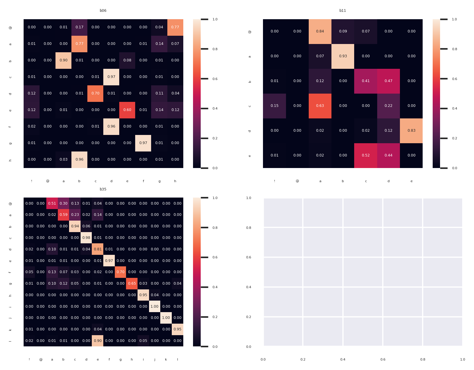
Comparing across birds we can see that some individuals have a very linear song with the most frequent transitions on the diagonal (like b35 in the bottom right), while others have more variable transitions (b17 in the bottom left).

Now you’ve seen a detailed example of using crowsetta to access and transform annotations in a specific format in order to fit a simple model of behavior.

---

[1]

Nicholson, D., Queen, J. E., & J. Sober, S. (2017). Bengalese Finch song repository (Version 7). figshare. https://doi.org/10.6084/m9.figshare.4805749.v7

[2]

Woolley SM, Rubel EW (1997) Bengalese finches lonchura striata domestica depend upon auditory feedback for the maintenance of adult song. J Neurosci 17: 6380–90.

[3] (1,2)

Honda E, Okanoya K (1999) Acoustical and syntactical comparisons between songs of the white-backed munia (lonchura striata) and its domesticated strain, the bengalese finch (lonchura striata var. domestica). Zool Sci 16: 319–326.

[4]

Jin DZ, Kozhevnikov AA (2011) A Compact Statistical Model of the Song Syntax in Bengalese Finch. PLOS Computational Biology 7(3): e1001108. https://doi.org/10.1371/journal.pcbi.1001108